Convolutional Neural Networks

From sports to medicine, transportation to security…
Have you ever wondered how a surveillance camera manages to recognize a face in a crowd, how a medical scanner detects a concealed tumor, or how a system tracks a train’s trajectory with millimeter precision?

Introduction

A Convolutional Neural Network (Convolutional Neural Network, or CNN) is a type of supervised deep learning algorithm that confers upon computers a form of “vision”: it can analyze and recognize objects in the visual world.

The Convolutional Neural Network (Convolutional Neural Network, CNN), by analogy, refers to the functioning of biological neural networks and consequently constitutes an extension of the Artificial Neural Network (Artificial Neural Network, ANN). Its applications are primarily found in image recognition and analysis.

Building upon the principles of linear algebra, and more particularly on matrix manipulation, convolutional neural networks apply convolution and transformation operations to detect and extract pertinent patterns within an image.

How CNNs Operate

The functioning of a Convolutional Neural Network (CNN) relies on an architecture composed of three principal layer types. These layers process spatially structured input data, such as images, audio spectrograms, or video sequences:

• Convolutional layer (Convolutional layer)
• Pooling or subsampling layer (Pooling layer)
• Fully connected layer (Fully connected layer)

Convolutional Layer

The convolutional layer constitutes the network’s core, where the majority of computations are performed. Its operation requires components such as:

• Input data
• Filter (kernel)
• Feature map

Operational Mechanism:

• Convolution (dot product)
• ReLU (eliminates negative values)
• Pooling (dimensionality reduction)
• Repeat these steps
• Final classification

Input Data: Consider an input image of size 24×24 pixels, which will be transformed into a 3D pixel matrix corresponding to the respective number of pixels in the image. This means that the input is represented in height, width, and depth corresponding to the RGB characteristics of the image.

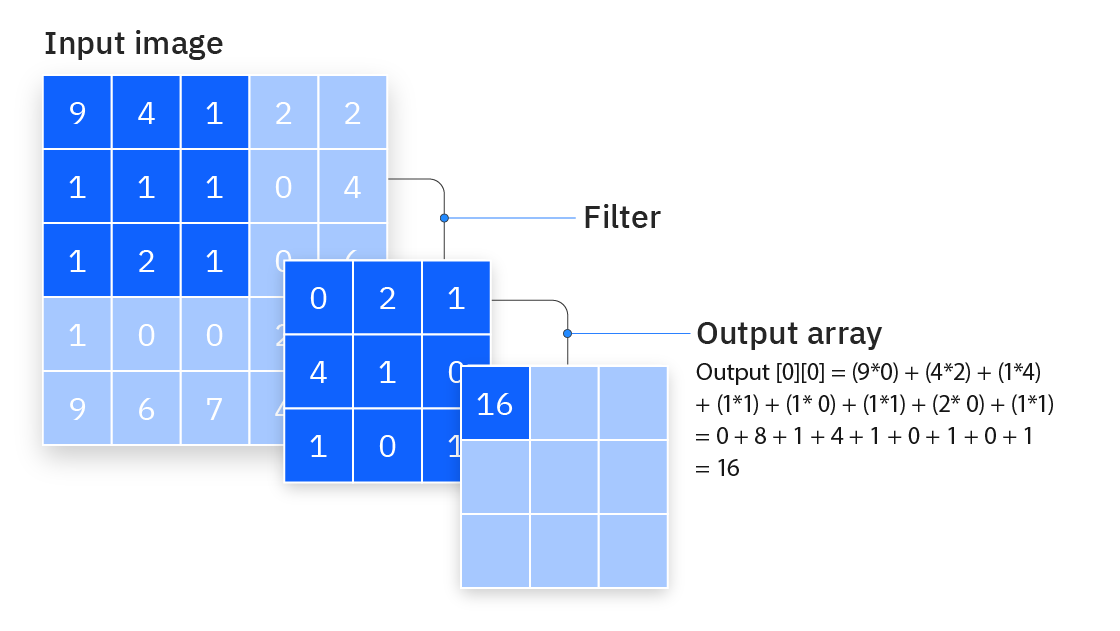
Filter (kernel): The filter is a weight matrix that traverses the image to detect shapes and characteristics. This process is known as the convolution operation.

• Contours
• Lines
• Textures
• Geometric shapes
• More complex characteristics in deeper layers

Its size may vary, although by default it is 3×3, there exist 5×5, or 7×7 pixel filters. The receptive field corresponds to the input image area that influences an output neuron.

The filter is positioned on an image region and the dot product is calculated based on the input pixels and the filter. This value is then saved in a feature map. Subsequently, the filter is shifted by one stride, repeating the process until the entire pixel surface of the image has been processed.

Certain filter hyperparameters remain fixed during the process, however the weights are adjusted to maximize performance via backpropagation and gradient descent operations. Three critical hyperparameters exist that are paramount in obtaining favorable results and that influence the output volume; they must be defined well before the process.

1. Number of filters: Affects the depth of the output. For example, three distinct filters would produce three different feature maps, thus creating a depth of three. Each filter acts as a specialized detector (contours, textures, shapes) and produces its own feature map; these maps stack to form the output depth.

2. Stride: Is the distance, or number of pixels, over which the kernel moves across the input matrix. While stride values of two or more are rare, a larger stride produces a smaller output. A stride of 1 means the filter moves pixel by pixel (detailed examination), while a stride of 2 skips one pixel with each movement (faster examination, smaller image).

3. Zero-padding: Is generally used when filters do not match the input image. This zeros all elements located outside the input matrix, producing a larger or equal-sized output. Three padding types exist:

   • Valid padding: This is also called the absence of padding. In this case, the last convolution is abandoned if dimensions do not align. (If the puzzle pieces don’t fit at the edge, they are abandoned)
   • Same padding: This padding guarantees that the output layer has the same size as the input layer. (Empty pieces are added around so everything fits perfectly)
   • Full padding: This padding type increases the output size by adding zeros to the input border. (Even more empty pieces are added to obtain a larger image)

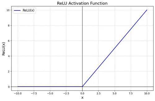
Following the convolution operation, the CNN immediately applies the ReLU function (Rectified Linear Unit). This activation function acts as a selective filter that eliminates weak signals (negative values) to retain only significant activations (positive values).

Operational Principle:

• Positive value → retained as is
• Negative value → transformed to zero

Formula: ReLU(x) = max(0, x)

Practical Example: Feature map before ReLU: [-2, 5, -1, 8, -3, 4] Feature map after ReLU: [0, 5, 0, 8, 0, 4]

Impact on Learning: The introduction of this non-linearity is crucial as it enables the network to model complex relationships between characteristics. Without ReLU, the CNN would be limited to linear transformations and could not detect sophisticated patterns such as spatial relationships between facial elements (eye-nose distance, mouth-cheek configuration) or other complex visual subtleties.

This step thus transforms a simple mathematical calculation into a genuine intelligent recognition process.

Additional Convolutional Layer

It is frequent that layer hierarchization is applied to progressively analyze the increasing complexity of an image. This cascade architecture enables the CNN structure to adapt intelligently: subsequent layers can exploit information from the receptive fields of preceding layers, thus creating a genuine detection hierarchy.

Characteristic Hierarchy Principle:

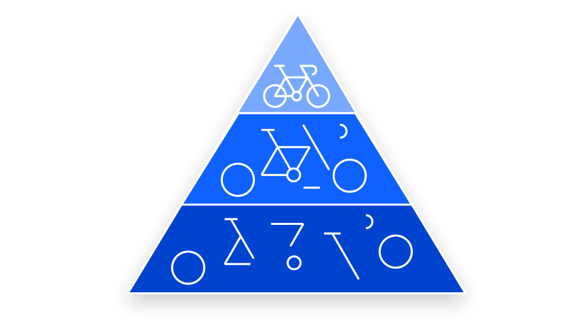
• Initial layers: Detect low-level characteristics (contours, lines, simple textures)
• Intermediate layers: Combine these elements to identify more complex shapes (angles, curves, geometric patterns)
• Deep layers: Recognize specific object parts (wheels, handlebars, frames)
• Final layers: Assemble these parts to identify the complete object (bicycle, car, face)

Concrete Example: Consider bicycle recognition. The CNN proceeds in stages:

1. Detection of circles and straight lines
2. Identification of circular shapes (potential wheels)
3. Recognition of handlebars and frame
4. Final association: “wheels + handlebars + frame = bicycle”

This hierarchical approach enables the network to construct a progressive understanding of the image, where each layer refines and enriches the analysis of the previous one. Ultimately, the convolutional layer converts the image into structured numerical values, enabling the neural network to interpret and extract pertinent patterns for final classification.

Pooling or Subsampling Layer (Pooling layer)

In this stage of the CNN process, the collected information is reduced and grouped to decrease data dimensionality. Following the same process as the convolutional layer, it applies a filter that, unlike the convolutional layer, has no weights. An aggregation function is applied to the receptive field values to populate the output array. This aggregation function constitutes the primary configurable parameter that determines the pooling type utilized.

Primary Objectives:

• Reduce data size
• Decrease the number of parameters
• Preserve important characteristics

The two principal pooling types (aggregation functions):

1. Max Pooling:

• Aggregation function: f(region) = max(values)
• Selects the maximum value in each receptive field region
• Preserves the most salient characteristics
• More commonly used as it preserves important contours and details

2. Average Pooling:

• Aggregation function: f(region) = average(values)
• Calculates the arithmetic mean of all values in the receptive field
• Smooths data by reducing noise
• Less utilized but useful for certain specific applications

Visualization

2×2 region organized as a matrix:

Calculations according to pooling type:

Max Pooling:

• We examine all values: 1, 3, 2, 4
• We take the largest: max(1, 3, 2, 4) = 4
• Result: 4

Average Pooling:

• We sum all values: 1 + 3 + 2 + 4 = 10
• We divide by the number of values: 10 ÷ 4 = 2.5
• Result: 2.5

Process Visualization:

The pooling filter “examines” this 2×2 region and summarizes it into a single value according to the chosen aggregation function.

These parameters (aggregation function type, filter size, stride) are configurable before training according to the model’s specific needs, enabling adaptation of pooling behavior to the targeted classification task.

Fully Connected Layer (Fully connected layer)

This layer performs classification based on characteristics extracted from previous layers and their filters. It applies an activation function (generally softmax) that enables data conversion to probabilities: each possible class receives a score between 0 and 1, and the sum of all probabilities equals 1.

Example:

For animal recognition:

• Cat: 0.7 (70% probability)
• Dog: 0.2 (20% probability)
• Bird: 0.1 (10% probability)
• Total: 0.7 + 0.2 + 0.1 = 1.0

The class with the highest probability (here “Cat” with 0.7) is the final prediction.

Conclusion

Convolutional Neural Networks (CNNs) constitute a particularly effective deep learning architecture for image processing and analysis. Their operation relies on three principal components: convolutional layers that extract characteristics, pooling layers that reduce dimensionality, and fully connected layers that perform final classification.

Architecture and Performance

This hierarchical structure enables CNNs to progressively detect increasingly complex patterns, from simple contours to complete objects. Configurable hyperparameters (number of filters, stride, padding) offer adaptation flexibility according to the specific needs of each application.

Practical Applications

CNNs currently find concrete applications in numerous sectors: medical diagnosis through imaging, automated surveillance systems, industrial quality control, and autonomous vehicles. Their capacity to efficiently process large quantities of visual data makes them an indispensable tool for these domains.

Technical Perspectives

The continuous optimization of CNN architectures, combined with improved computational capabilities, enables envisioning more complex applications and increased precision in image recognition tasks. Understanding these fundamental mechanisms remains essential for effectively developing and implementing these technological solutions.